In any livestock system, the final stage of production, harvesting or marketing, is where biological performance becomes economic reality. Yet marketing decisions are often treated as fixed and uniform, as if every pig delivers the same value per kilogram. In practice, nothing could be further from the truth.
Because pigs differ in growth rate, feed conversion, health status, and mortality risk, each kilogram carried by each pig has a different cost.

And because packers apply premiums and discounts based weight and carcass quality, each kilogram also earns a different price.
The result is simple but powerful:
Every pig carries a unique profit profile; therefore, each kilo has a unique value.
This final article in the series introduces precision harvesting, a system looking to market pigs at their maximum economic value, not just their final live weight by:
- tracking those per-kilo profit differences
- visualizing them
- using the resulting insights to define the optimal time to market the animals.
Why profit per kilo varies?
Traditional thinking assumes that once a pig reaches market weight, every additional kilogram adds about the same amount of profit. But three forces break this assumption:
1. Cost per kilo changes as pigs grow
Earlier in finishing, growth rates accelerate so marginal gain to profit is highly efficient. As the pig matures, growth rates and subsequently marginal profit begins to decrease because:
- It stays in the barn longer increasing overhead allocation (utilities, labor, depreciation)
- It consumes more feed per kilogram of gain
This is particularly true for pigs with below average growth performance because not only are the above factors more significant, but it also occupies a space that could be occupied by a more efficient pig. Therefore a “cheap kilo” at 110 kg may become an “expensive kilo” at 130 kg.
2. Mortality affects cost structure
A pig that dies late in finishing carries enormous cost because most expenses have already been incurred. The surviving pigs must “absorb” those losses.
This inflates the cost per kilogram in the final group, often significantly.
3. Packers do not pay equally for all kilos
Premium and penalty grids based around weight bands, lean percentages and fat depths all mean that:
- Some kilos earn more
- Some kilos earn less
- Some kilos actively lose money
When you combine variable cost per kilo with variable value per kilo, you end up with a profit curve that rises, peaks, and eventually declines. Even producers not selling on a matrix still face variable costs per kilo, so profit per kilo is also variable.
The goal of precision harvesting is to identify this peak and harvest pigs when they reach it.
The core tool: tracking each pig’s “story”
Precision harvesting relies on one basic principle:
You cannot optimize profit until you measure variation.
All you need to begin is:
- Individual (or small-group) weights
- A good estimate of feed consumed at various intervals in finishing
- Average mortality timing
- Your slaughterhouse’s premiums and discounts
- A simple spreadsheet
With these, you can build two extremely useful visual tools: a profit frontier and a pig-level harvest map.
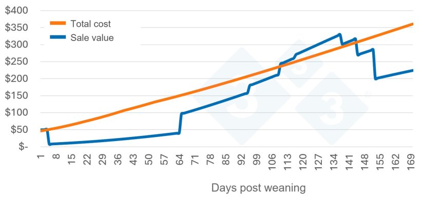
Tool 1: The profit frontier
A profit frontier is a curve showing:
- The estimated cost to produce each additional kilogram
- The expected price for those kilograms
- The resulting profit (or loss) per kilogram across the weight range
Producers can build a basic version with three steps:
Step 1: Estimate cost per kilo across the finishing period
Your spreadsheet might look like:
| Weight range | FCR | Total cost per Kg gain |
|---|---|---|
| 80–100 kg | 2.5 | Low |
| 100–115 kg | 2.9 | Medium |
| 115–130 kg | 3.4 | High |
Include mortality impact by adding a prorated cost per surviving pig and calculate a daily marginal total cost curve.
Step 2: Overlay the pig’s value curve
This may include:
- Sale value based on weight
- Slaughterhouse adjustments to price
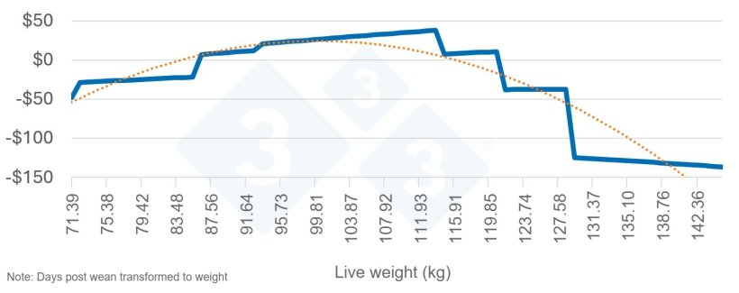
Step 3: Plot profit per kilo at each weight point
You'll typically see a shape like:
- Rising profit as pigs approach ideal harvest weight
- A plateau near maximum profit
- A decline as feed efficiency drops and packer penalties increase
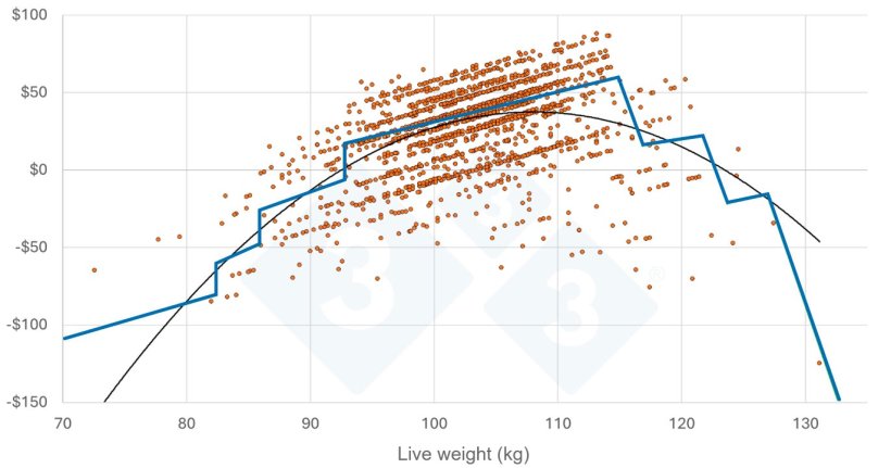
This curve shows the economic harvest point, not the biological one. You can even overlay actual marketing results on this curve to see how close your results are to optimal (Figure 3).
Tool 2: Pig-Level harvest map
This tool takes the frontier a step further by placing each pig on the grid, showing:
- Number of pigs that were marketed in that grid coordinate
- Average profit for those pigs
- Where profit was left on the table
| Carcass weight (kg) - Slaughterhouse price adjustments | |||||||||||
|---|---|---|---|---|---|---|---|---|---|---|---|
| ≤49 | 50 | 55.1 | 60.1 | 65.1 | 70.1 | 75.1 | 80.1 | 85.1 | ≥90.1 | ||
| Backfat Depth | ≤6 | 77% | 86% | 86% | 97% | 100% | 100% | 100% | 91% | 77% | 53% |
| 7 | 77% | 86% | 86% | 97% | 100% | 100% | 100% | 91% | 77% | 53% | |
| 8 | 77% | 86% | 86% | 97% | 100% | 100% | 100% | 91% | 77% | 53% | |
| 9 | 77% | 86% | 86% | 97% | 100% | 100% | 100% | 91% | 77% | 53% | |
| 10 | 77% | 86% | 86% | 97% | 100% | 100% | 100% | 91% | 77% | 53% | |
| 11 | 77% | 86% | 86% | 97% | 100% | 100% | 100% | 91% | 77% | 53% | |
| 12 | 77% | 86% | 86% | 97% | 100% | 100% | 100% | 91% | 77% | 53% | |
| 13 | 72% | 81% | 86% | 86% | 100% | 100% | 100% | 81% | 72% | 53% | |
| 14 | 72% | 81% | 86% | 86% | 100% | 100% | 100% | 81% | 72% | 53% | |
| 15 | 67% | 77% | 81% | 81% | 91% | 91% | 86% | 72% | 63% | 53% | |
| 16 | 67% | 77% | 81% | 81% | 91% | 91% | 86% | 72% | 63% | 53% | |
| 17 | 67% | 77% | 81% | 81% | 91% | 91% | 86% | 72% | 63% | 53% | |
| 18 | 67% | 77% | 77% | 77% | 81% | 81% | 81% | 72% | 53% | 53% | |
| 19 | 67% | 77% | 77% | 77% | 81% | 81% | 81% | 72% | 53% | 53% | |
| 20 | 67% | 77% | 77% | 77% | 81% | 81% | 81% | 72% | 53% | 53% | |
| ≥21 | 63% | 72% | 77% | 77% | 81% | 81% | 77% | 72% | 53% | 53% | |
| Carcass weight (kg) - Number of pigs | |||||||||||
|---|---|---|---|---|---|---|---|---|---|---|---|
| ≤49 | 50 | 55.1 | 60.1 | 65.1 | 70.1 | 75.1 | 80.1 | 85.1 | ≥90.1 | ||
| Backfat Depth | ≤6 | 1 | 1 | 6 | 12 | 30 | 22 | 9 | 1 | ||
| 7 | 13 | 32 | 124 | 146 | 31 | 4 | |||||
| 8 | 5 | 40 | 182 | 261 | 94 | 17 | 1 | ||||
| 9 | 1 | 4 | 38 | 204 | 333 | 122 | 23 | 4 | |||
| 10 | 6 | 43 | 171 | 360 | 144 | 26 | 4 | ||||
| 11 | 1 | 7 | 29 | 135 | 300 | 112 | 28 | 6 | 2 | ||
| 12 | 2 | 18 | 139 | 235 | 107 | 18 | 4 | ||||
| 13 | 1 | 13 | 154 | 347 | 136 | 27 | 3 | 1 | |||
| 14 | 2 | 27 | 40 | 32 | 9 | 3 | 2 | ||||
| 15 | 2 | 19 | 42 | 24 | 3 | 1 | 1 | ||||
| 16 | 3 | 13 | 31 | 18 | 4 | 1 | |||||
| 17 | 1 | 9 | 19 | 17 | 7 | 1 | |||||
| 18 | 4 | 16 | 6 | 3 | 1 | ||||||
| 19 | 1 | 7 | 2 | 1 | |||||||
| 20 | 1 | 2 | 4 | 1 | 1 | ||||||
| ≥21 | 5 | 1 | |||||||||
| Carcass Weight (kg) - Average per head profit ($) | |||||||||||
|---|---|---|---|---|---|---|---|---|---|---|---|
| ≤49 | 50 | 55.1 | 60.1 | 65.1 | 70.1 | 75.1 | 80.1 | 85.1 | ≥90.1 | ||
| Backfat Depth | ≤6 | -130.67 | -44.99 | -67.20 | -8.39 | 13.35 | 34.85 | 36.10 | -14.88 | ||
| 7 | -53.83 | -6.73 | 12.81 | 29.36 | 39.44 | 14.79 | |||||
| 8 | -47.80 | -16.05 | 16.19 | 30.93 | 45.59 | 17.31 | 6.40 | ||||
| 9 | -105.80 | -23.20 | -8.64 | 21.15 | 33.99 | 47.45 | 18.08 | -6.07 | |||
| 10 | -50.89 | -2.13 | 23.02 | 37.15 | 48.75 | 37.22 | 9.50 | ||||
| 11 | -64.60 | -62.60 | 1.22 | 24.93 | 38.94 | 50.49 | 38.81 | -0.48 | -76.07 | ||
| 12 | -31.30 | -2.15 | 26.49 | 41.15 | 54.73 | 28.48 | -9.72 | ||||
| 13 | -96.96 | -39.97 | 23.28 | 42.10 | 56.69 | 2.48 | -24.76 | -88.53 | |||
| 14 | -34.34 | 20.11 | 40.46 | 44.30 | -1.99 | -7.81 | -100.44 | ||||
| 15 | -37.49 | -5.22 | 14.55 | 5.73 | -27.71 | -67.00 | -107.92 | ||||
| 16 | -43.18 | 2.65 | 15.50 | -0.45 | -26.39 | -48.81 | |||||
| 17 | -91.03 | -0.48 | 17.74 | 12.86 | -29.77 | -34.20 | |||||
| 18 | -32.75 | -19.47 | -14.83 | -31.40 | -81.98 | ||||||
| 19 | -28.14 | -4.20 | -9.88 | -66.90 | |||||||
| 20 | -26.75 | -40.25 | -19.99 | 17.77 | -19.31 | ||||||
| ≥21 | -16.74 | -34.88 | |||||||||
To build it:
- Record the weight and carcass quality of each pig at slaughter.
- Count pigs that land in each category
- Estimate cost per pig based on its growth history or group average.
- Subtract cost from premium or penalty adjusted revenue.
You will quickly see:
- Opportunities to adjust marketing strategies
- Uniformity (or lack of it) explains where big improvements to profitability can be made
- Can quickly calculate the value of reducing variation
Even without a formal packer matrix, this methodology still works because cost per kilo is never uniform.
Turning insight into action
Once you build these plots, precision harvesting becomes a practical decision-making tool.
Producers gain the ability to:
- Market pigs based on profit, not weight, as the profit optimal point changes with prevailing market conditions
- Reduce off-target penalties
- Identifying when pigs can be marketed early to improve barn turnover
- Identify barns or systems with costly late growth
- Target interventions for pigs at risk of producing “expensive kilos”
In short, precision harvesting converts information into profit by pushing as many kilos as possible into the profit maximum zone.
Closing thought
In Part 1, we learned that what you put into pigs determines what you get out.
In Part 2, we showed that precision tools amplify the value of that investment.
In Part 3, precision harvesting ties it all together by ensuring you capture the profit you worked so hard to create.
Because when every pig grows differently, every kilo has a different value, and the producer who recognizes this is the producer who captures more of the value already present in their system.
Watch the free webinar “Precision Production of Pigs – Unlocking Profitability Through Managing Variation” to learn more about actionable strategies to reduce variation, improve carcass value, and enhance overall farm profitability.